These are the pages relevant to the topic of factor analysis:  Regression.  Introduction to principal components analysis.  Orthogonal factor rotation.  This page, Oblique rotation.  Full factor extraction.  Principle Axes extraction.  Cluster analysis.

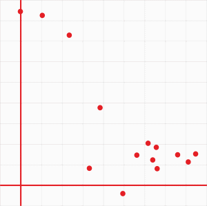
Factor analysis: Introduction to oblique rotation

In our introduction to PCA, we extracted two components from the correlation matrix, and agreed that these two components had non-obvious interpretations.  Part of the difficulty was due to the variables not clearly clustering on one or other component, so we rotated the component axes orthogonally.  Clustering on one or other component axis improved, but still remained unclear.  Figure 1 shows the orthogonal rotation.

Figure 1.  Orthogonal rotation of two components

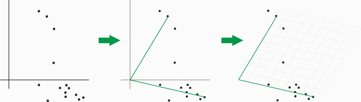
We wish to rotate the axes so that an axis more clearly lies on or intersects a cluster of variables.  To do that, we remove the constraint that the axes are at right angles.  The consequence is that the obliquely rotated components are no longer independent and uncorrelated, but instead show a degree of correlation.  Lets see how that works.  Figure 2 shows the two components as extracted on the left, two axes placed through the two apparent clusters of variables in the centre, and a grid placed over the results on the right, oriented according to the oblique axes.  Voila, an oblique rotation.

Figure 2.  Oblique rotation of two components

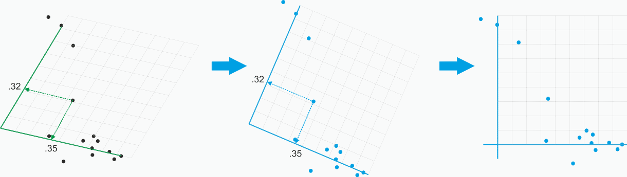
To give a more conventional view of the rotation, the grid of the right-hand plot in Figure 2 is adjusted to Cartesian coordinates.  When viewing the resulting plot, you must keep muttering to yourself, "the axes are shown at right angles, but the components they represent are in fact at an angle".  Figure 3 shows the presentation of the oblique components as a Cartesian plot.  The change is purely for presentation;  the loadings have not changed.

Figure 3.  Oblique rotation presented in conventional in Cartesian view, the loadings do not change

The pattern matrix

The loadings of the variables on the two oblique components are shown in Table 1, called the "Pattern Matrix".

Table 1.  Pattern matrix of obliquely rotated components

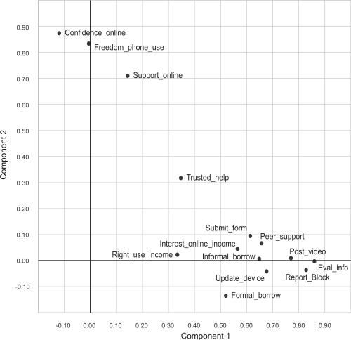
Figure 4 shows a plot of the pattern matrix loadings.

Figure 4.  Annotated plot of the pattern matrix

The pattern matrix loadings are the correlations between the variables and the oblique components which express the unique variance that the variable accounts for in the corresponding component.  These pattern matrix loadings are the exact equivalent of Beta weights in a regression.  We recall that the Beta weight in a regression equation expresses the unique contribution of an IV to the DV, and when squared gives the % of variance in the DV that is accounted for by the IV.

Table 2 shows the square of the pattern matrix loadings.

Table 2.  Pattern matrix loadings squared and summed

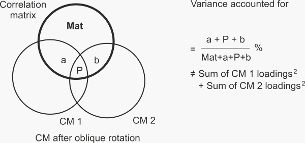
Our interest is in the total of the squared loadings -- that is, the total variance uniquely accounted for by the obliquely-rotated components.  We recall that the total squared loadings for the orthogonally rotated components were 4.48 and 2.25, summing to 6.73.  Any rotation redistributes the variance accounted for, so the change for oblique components is to be expected.  However, we note that the summed loadings for the orthogonal rotation, 6.73, is different from the sum for the oblique rotation, 6.66.  (We note that the squared loadings for the extracted components, before rotation, also sum to 6.73.)

A Venn diagram is useful to illustrate the variance accounted for in the correlation matrix, as in Figure 5.

Figure 5.  Venn diagram of the variance accounted for in the correlation matrix by oblique components

The pattern matrix loadings on an oblique component relate to the unique variance that the component accounts for -- region "a" for Component 1, and region "b" for Component 2.  Because the two components are correlated, there is variance, P, that they share which also accounts for variance in the correlation matrix, but P is excluded from the loadings.  This means that the pattern matrix loadings are equivalent to the way Beta weights (§1) in a regression analysis identify unique variance shared between the IVs and the DV.  The loadings shown in the pattern matrix, Beta weights, are given by the ratio of their unique contribution, "a", to the variance of the correlation matrix represented by "Mat + a".  Now may be a good time to refer to Figure 3 in the Regression page which also illustrates other kinds of correlations (variance ratios).  Glance at Figure 2 as well there (§1).

(§1) We might have mentioned this before.  It becomes important if we wish to better understand the Structure Matrix, a topic in oblique rotation arriving shortly.

The correlation between the oblique components, an output from your statistics software, is shown in Table 2.

Table 2.  Component correlation matrix

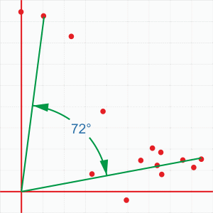
The two obliquely-rotated components correlate r = .31.  Figure 6 illustrates the oblique component axes laid onto the plot of the orthogonal (Varimax) rotation and shows the angle between them, 72°.  We recall that the cosine of the angle between two axes is equal to their correlation, hence Cos(72°) = .31.

Figure 6.  Correlation (angle) between oblique components

Some details on oblique rotation

As for orthogonal rotation, the oblique axes are calculated by an iterative algorithm, and there is a variety of rotation algorithms.  The most common oblique rotation algorithm is "Oblimin".  It is also an implementation of the concepts of coupling and cohesion, but where coupling is given much greater attention.  As in "Varimax", component axes are rotated in small increments, and at each increment the algorithm checks if the cohesion of the variables on each component has increased.  We recall that cohesion is measured by the variance of the squared loadings. The algorithm becomes "Oblimin" by the addition of a second criterion, which is the minimisation of the squared loadings accounted for by the other components.  That is, the coupling between components is minimised.  The algorithm terminates when cohesion suffers as coupling reduces, or when coupling suffers as cohesion increases.

As for orthogonal rotation, it is routine to specify "Kaiser Normalization".  Normalization scales component loadings by the square root of the variable's communality.  This weights each variable equally so that variables with high communalities (and hence high loadings) do not disproportionately dominate the rotated solution.

The structure matrix

We now need to account for the fact that the variance in the correlation matrix which is accounted for by the pattern matrix loadings is not what we were expecting.  Our two extracted components (and the two orthogonally rotated components) have summed squared loadings equal to 6.73, while this is 6.66 for the obliquely-rotated components.

Well, it is not necessary to understand this apparently missing variance.  You will be able to interpret oblique rotations and obliquely rotated components perfectly well by considering the pattern matrix only;  it is after all exactly what you are looking for in better showing clusters of variables by allowing correlated components.  On the other hand, some external examiners can be rather awkward if they sense that you do not have a total command of the technique which underpins your entire thesis....  Without putting too fine a point on it, that may well be a good enough reason to restrict yourself to orthogonal Varimax rotation.

The structure matrix loadings of the variables on the two oblique components are shown in Table 3.

Table 3.  Structure matrix of obliquely rotated components

The loadings shown in the structure matrix are correlation coefficients.  Refer to Figure 3 in the Regression page if necessary to see that a correlation corresponds to the variance ratio of "a + P" to "Mat + a + P + b" illustrated in the Venn diagram of Figure 5 above, while a Beta weight is congruent with the ratio "a" to "Mat + a".  The missing variance lies in region "P".  To get that missing shared variance P back into the complete account for variance we must use the entries -- correlations -- from the structure matrix.

Specifically, we refer to Figure 2 in the Regression page which showed us how to similarly account for missing variance when trying to account for R² in a regression analysis by only looking at the Beta weights.  We found out that the Beta weights must be multiplied by the correlations.  Here, it turns out that the pattern matrix loadings must be multiplied by the structure matrix loadings -- the pattern matrix is a matrix of Beta weights, while the structure matrix is a matrix of correlation coefficients.  The calculations to show the full accounting of the oblique components for the variance in the correlation matrix is shown in Table 4.

Table 4.  Product of pattern and structure matrix loadings

Interpreting the obliquely rotated components

As with any table of factor loadings, we highlight loadings above some criterion value such as 0.4, and sort the table in descending order.  We usually interpret the pattern matrix, its edited and sorted version is shown as Table 5.

Table 5.  Pattern matrix loadings edited and sorted

The oblique components show a clearer structure, reasonably obvious in Figure 4.  Each variable only has one substantial loading on one component, except for two variables which do not have a substantial loading on any component.

Two difficulties remain.  One is that, as with the components when extracted or orthogonally rotated, Component 1 seems to comprises a rather mixed bag of variables, Component 2 is clearly a separate cluster of variables but also is somewhat mixed, and two variables do not feature in the results.  The oblique rotation of just two components seems inadequate, so the next section will rotate four components obliquely.

The second difficulty is knowing what to do with the fact that the two components are correlated.  This difficulty is partly related to the apparent inadequacy of having just two components, as above.  More importantly, however, it is a difficulty inherent in oblique rotation.  Orthogonal components are easier to interpret because they are, by definition, separate, unrelated, and independent.

Our discussion so far has been concerned with PCA -- Principle components analysis -- and has treated the topics of orthogonal and oblique rotation in this context.  After considering the analysis of four factors, we will introduce Principle axes analysis, which many consider to be "Factor Analysis" proper.

©2025 Lester Gilbert