This page introduces hierarchical cluster analysis using Ward's method, illustrated in SPSS.  It is intended to complement the pages dealing with Factor Analysis, illustrating an alternative and usually very interesting view of the clusters of variables that might be found in a correlation matrix.

The context and example data used here is given in the page which introduces Principle Components Analysis.  We reproduce the correlation matrix as Table 1.

Table 1.  Correlation matrix

There are a number of clustering algorithms and a number of methods of presenting clusters.   I have found the following protocol the most useful for the kinds of research questions which might suggest regression or factor analysis involving observational data.  We will investigate hierarchical clustering of the 14 variables in the correlation matrix (§1), so the first step is to select "Hierarchical Cluster" from the SPSS "Classify" menu.  Select "Variables" in the dialogue box, and uncheck "Statistics", they are interesting but like the correlation matrix are more or less un-interpretable without a visual plot.  In the "Plots" menu, select "Dendrogram" and select "None" for icicle plots (§2).

The major choices are the selection of method and the selection of measures.  I've played with them all at one time or another, and keep returning to Ward's Method using Squared Euclidian distances (§3).

(§1)  The other possibility is to investigate the clustering of the 180 data rows that gave rise to the correlations, that is, the participants in the study.  Not in the scope of our current interest.

(§2)  I have nothing against an icicle plot, but the SPSS implementation seems rather crude.  Leave the selection at default if you wish and see if you agree.

(§3)  You can have great fun dropping into some deep rabbit holes while interpreting and comparing all the other methods and measures.  Try it and see if you always come back to Ward's method and Squared Euclidian distances.

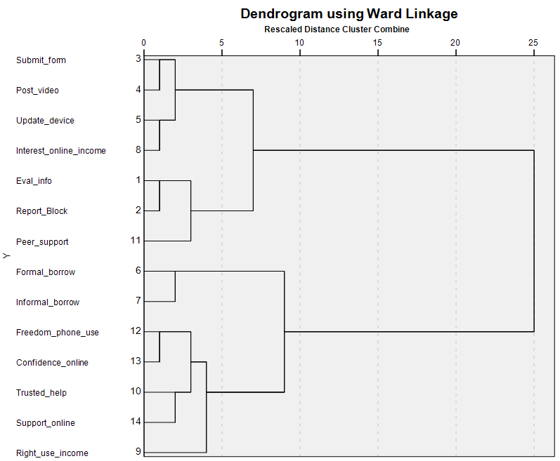
Cluster analysis of Table 1

The output of most interest is the dendrogram plot, shown as Figure 1.

Figure 1.  Dendrogram plot

We initially work from the right-hand side of the dendrogram for the big picture.  At distance "25" (§4) all the variables cluster into one.  Before that, we see that there are two clusters of variables, one formed at distance "7" and the other at distance "9".  In turn we can distinguish four earlier clusters, and give them working titles of A, B, C, and D.  Now working from the left-hand side, we see that variables 3, 4, 5, and 8 form cluster A at distance "2", variables 1, 2, and 11 form cluster B at distance "3", and these two join at distance "7".  Variables 6 and 7 form cluster C at distance "2", and variables 9, 10, 12, 13, and 14 form cluster D at distance "4", these two combining at distance "9".  We could be tempted to examine cluster D and discern two sub-clusters.  Cluster D1 comprises variables 12 and 13 at distance "1", while cluster D2 comprises variables 10 and 14 at distance "2".  It is variable 9 which joins D1 and D2 at distance "4".

(§4)  Distances are in quotes because they have no intrinsic meaning.  They simply provide a scale 1 to 25 on which to arrange the variables, and then the clusters of variables as they form, from closely connected to distantly connected.

Interpreting cluster A suggests it comprises technological ability (variables 3, 4, 5) which seem to provide the primary connection with interest in online income (variable 8).  Cluster B addresses security (variables 1 and 2) with peer support that helps with this (variable 11).  Cluster C comprises finances (variables 6 and 7).  Cluster D comprises social D1 freedom and confidence (variables 12 and 13) and social D2 help and support (variables 10 and 14), joined by use of income (variable 9).  The super-cluster A+B combines technology ability with technology security, and C+D combines the social matters, finances on the one hand with freedom, confidence, help, and support.  The two super-clusters thereafter maintain their separation to the end of the analysis.

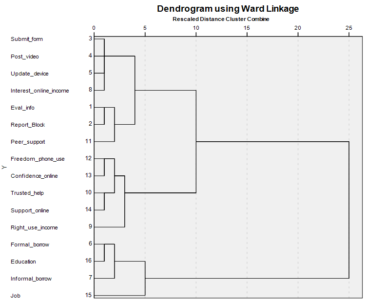
Cluster analysis of Table 1 with marker variables

We introduced marker variables in the discussion of Principle Axes factor analysis.  We can place the three markers of interest (Job, Education, Age) into the correlation matrix and see how the cluster analysis deals with them.  The first finding is that the inclusion of Age renders the cluster analysis meaningless -- every variable clusters at distance "1", and Age joins them at distance "25".  This is the cluster analysis's way of saying that Age has so little to do with any of the variables that they cannot be separated.  We re-run the analysis after removing Age, and obtain Figure 2.

.

Figure 1.  Dendrogram plot with marker variables

The addition of Job and Education changes the cluster picture.  Clusters previously labeled A, B, and D remain substantially as they were, these three clusters joining together at distance "10".  Cluster C, finances, gains first Education and then Job and in doing so becomes a super-cluster at distance "5", remaining separate until the end of the analysis.

©2025 Lester Gilbert