This is a refresher page on multiple linear regression, created as a reference for the pages which introduce factor analysis.  It is not a complete introduction to MLR.

Introduction

Multiple linear regression (MLR) is a technique which identifies the variation seen in one variable, the dependent variable or DV, with variation seen in two or more other variables, the independent variables or IVs.  This is usually interesting if we want to know about the contributions made by the IVs to the DV.

We begin with a specific example, using data from a research project investigating the variables which support individual online commerce -- in current vernacular, a "side hustle".  Participants were asked about their interest in generating income through online activities, and completed a survey which asked further questions about their online and commercial abilities and experiences, listed in Table 1.  Our research question is which of these variables are most closely associated with interest in online income.

Table 1.  Abilities, experiences, supports

MLR starts from the correlation matrix of the DV and IVs.  In Table 2 we reproduce the correlations between the DV and the IVs only, and not the entire matrix showing the inter-correlations between all the variables.

Table 2.  Correlations with DV

Note:  * and ** – Significant at .05 and .01 respectively

Our interest is in establishing which IVs are significantly associated (§1) with the DV.  From Table 2, we may be tempted to say that most (10 out of 13) of the IVs are significantly associated with the DV, being Evaluate info, Report or Block, Submit forms, Post videos, Update device, Informal borrow, Right to use income, Peer support, Freedom of phone use, and Support online participation;  and that only Formal borrow, Trusted help, and Confidence online are not significantly associated.  We may also be tempted to say that the five most significant IVs, for example, are those with the highest correlations with the DV, being (in descending order) Update device, Evaluate info, Submit forms, Report or Block, and Post videos.

We would be wrong.

(§1) Just a reminder.  When interpreting correlations, we may wish to claim one or other of the IVs predict, support, explain, verify, underpin, etc, the DV.  But we know that such claims are not justified by the statistical analysis in itself.  Instead, it is the research circumstances and protocol which give substance to such claims.  It is common to find MLR presented in statistics texts and tutorials as a technique of prediction with the IVs termed predictors and the regression equation called the prediction equation.  More careful language, however, is needed when an MLR is presented in a conference paper or journal article.

Simple linear regression

The IV which is most associated with the DV is the one with the largest correlation, "Update device" with r = .55 in our example.  We recall that r² represents the shared or common variance between two correlated variables, hence we interpret the r of .55 as showing that "Interest in online income" and "Update device" have approximately 30% variance in common.  SPSS gives us the details for this SLR, called Model 1, as follows in Table 3.

Table 3.  SLR statistics, one IV

Dependent Variable: Interest in generating income through online activities

In the case of SLR -- one IV -- we recognise the coefficient of regression, R, as being equal to the correlation, r, and we notice that the Beta weight is also equal to r.  The IV "Update device" is a highly significant associate of the DV, t = 8.82 and p < .001.  In standardised units, we can construct the regression equation, shown as Eqn 1:

Eqn 1.    Predicted interest in generating income through online activities = 0.55 × Ability to update own mobile phone, tablet, or computer

We can understand the regression equation as constructing a hypothetical variable from the IV or IVs, called "Predicted DV".  This hypothetical variable is constructed (a) so that it correlates maximally with the DV itself, and (b) no other construction has a higher correlation.

Multiple linear regression

We now ask which other IVs share significant variance with the DV.

MLR identifies the next IV as the one sharing the most "left over" variance with the DV.  That is, having accounted for the shared variance shown by the IVs so far, MLR seeks the next IV which accounts for as much as possible of the variance not yet accounted for.

In SPSS we request a "Forward" or "Stepwise" regression method and set .05 as the desired level of significance for inclusion.  This method adds the IVs one at a time, and stops when no further IV makes a significant contribution.  (An SPSS regression method called "Enter" adds all the IVs at once into the regression equation, and we'll look at that later.)

Here we consider the regression with two IVs. Table 4 provides the details for the result, called Model 2.  The analysis has added the variable, "Ability to evaluate whether online information is trustworthy".

Table 4.  MLR statistics, two IVs

Dependent Variable: Interest in generating income through online activities

We notice that the two IVs, taken together, account for 35% of the variance in the DV, an increase of 5% from Model 1.  The regression equation in standardised units is now Eqn 2:

Eqn 2.    Predicted interest in online income = 0.42 × Update device + .26 × Evaluate info

Our hypothetical variable "Predicted DV" correlates R = .59 with the DV, accounting for 35% of its variance. 

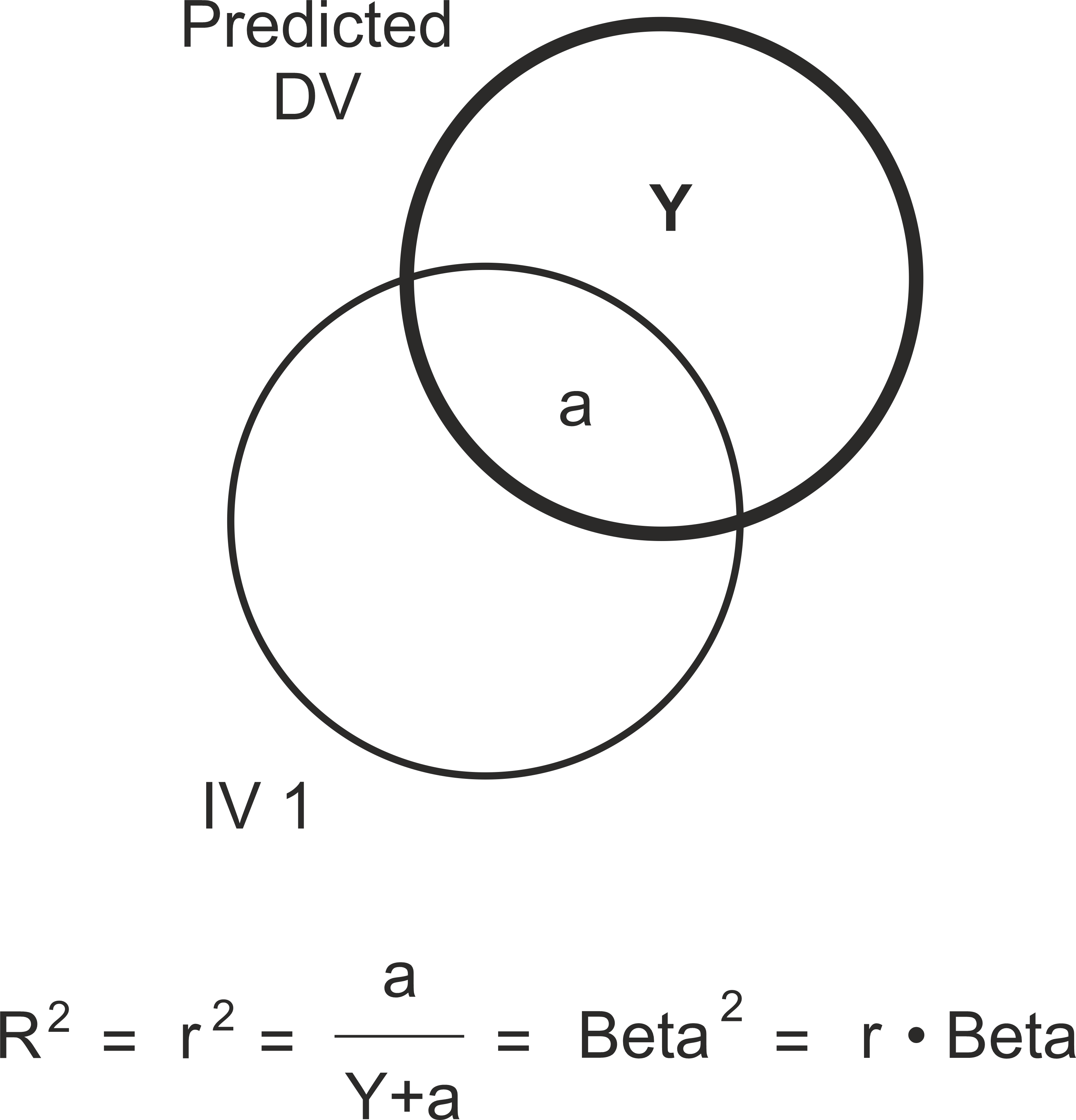
Partial correlation

We pause our pursuit of the IVs which are significantly associated with the DV in order to better understand the development of the regression when moving from the SLR Model 1 with one IV to the MLR Model 2 with two IVs.

We notice that the beta weight for Update device (we'll call this "IV 1") in Model 1 is .55, while in Model 2 it is .42.  Why the change?  A beta weight is conveniently interpreted as a correlation coefficient, and hence IV 1 correlates .55 with the Model 1 variable "Predicted DV" while it correlates .42 with the Model 2 variable "Predicted DV".  Similarly, while the correlation of Evaluate info (we'll call this IV 2) with the DV is .47, its correlation (beta weight) is .26 with the Model 2 "Predicted DV".  There is no change to the correlation of IV 1 with the DV itself, it is still .55, and IV 2 still correlates .47 with the DV itself, but when put together in a regression equation for the Predicted DV their relationships change.  The introduction of IV 2 into the Model 2 Predicted DV regression equation results in a drop in the variance that IV 1 accounts for in the Predicted DV (§2) because it now shares some of this variance with IV 2. 

Figure 1 illustrates the relationships of the shared variances in Model 1 by way of overlapping circles (a Venn diagram).  The variance in common between IV 1 and the Predicted DV is shown as the region "a", while region "Y" represents unexplained variance in the Predicted DV, hence the total variance in the Predicted DV is "Y + a".  R² for Model 1 is 30%, region "a".

Figure 1.  Model 1 Venn diagram of variances in common, one IV

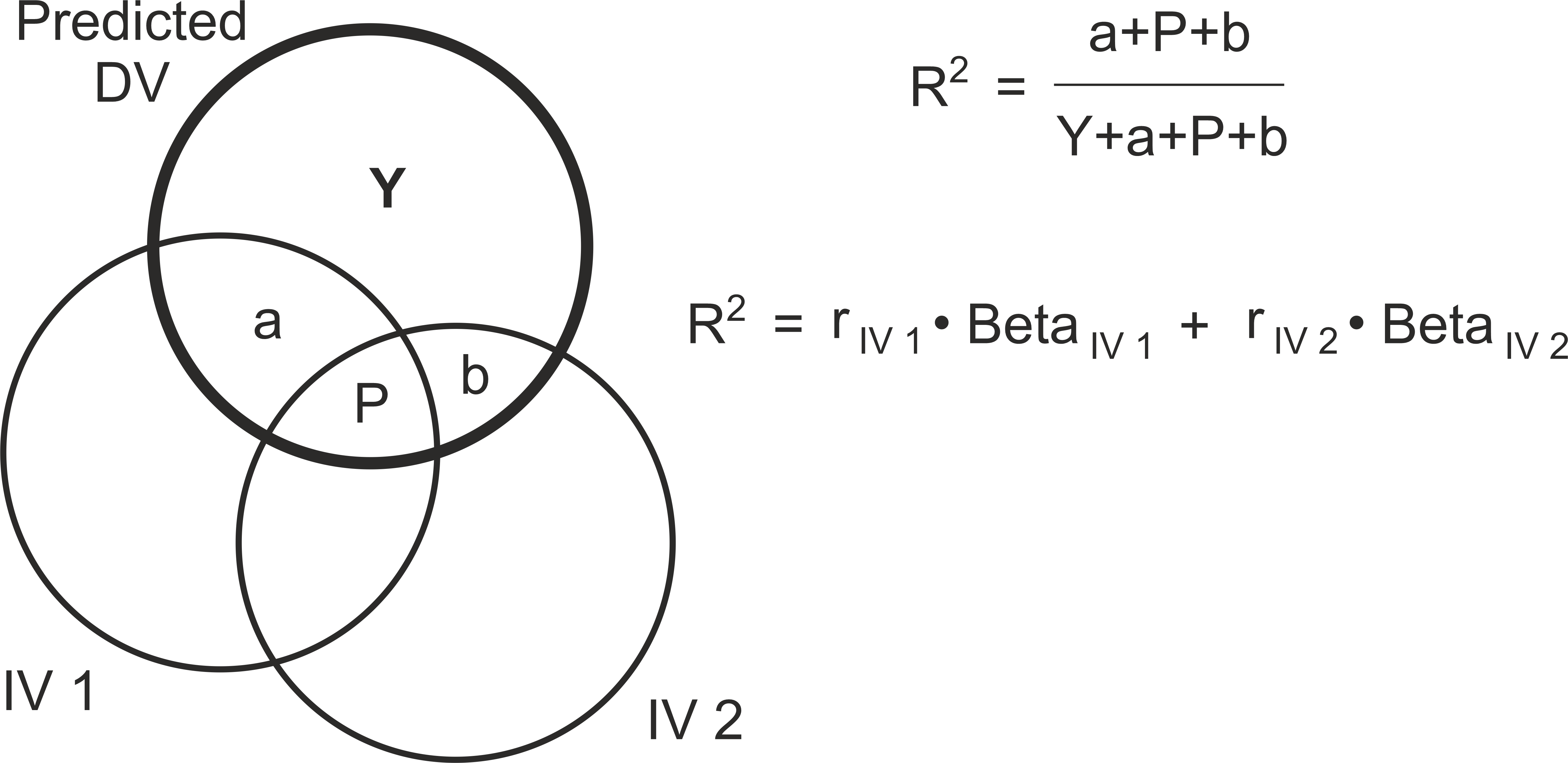
With one IV,  we know that R² = r² = Beta²;  but we might not have known that, strictly speaking, actually R² = r x Beta.  This will become important when there is more than one IV.

Figure 2 illustrates the relationships of the shared variances in Model 2.  The regions of variance accounted for by the two IVs are "a", "P", and "b".  Notice how region "a" of Model 1 is not the same size as region "a" of Model 2;  what was "a" in Model 1 is now "a + P" in Model 2.  The unique contribution of IV 1, "a", is smaller in Model 2 than it was in Model 1.

In relation to the total variance of the Predicted DV, Y+a+P+b, the regions accounted for by the IVs are a+P+b and this is R² for Model 2, 35%.  It is common, and reasonable, to suggest that Beta² for IV 1, (.42)² = 18%, represents the variance which IV 1 accounts for in the Predicted DV, region "a", and Beta² for IV 2, (.26)² = 7%, represents the variance which IV 2 accounts for in the Predicted DV, region "b".  These two values when added up give 25%, but we know that R² is 35%.

Figure 2.  Model 2 Venn diagram of variances in common, two IVs

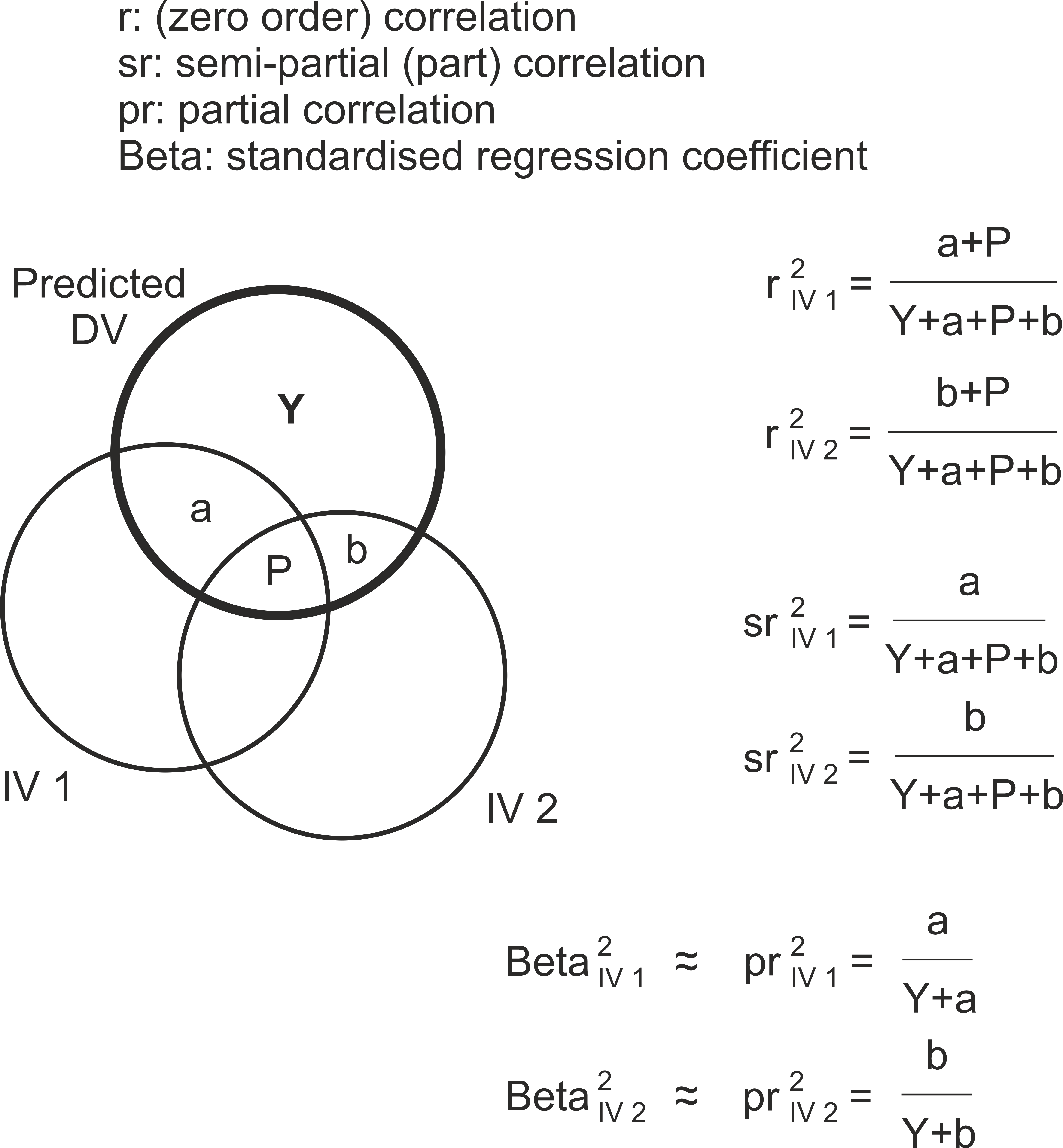
Beta for IV 1 represents the unique contribution of IV 1 towards the Predicted DV, and similarly for Beta for IV 2, but when added up these representations ignore their own common variance, region "P", which also contributes to the Predicted DV.  If we want to add up Beta weights so the result equals R², we need to weight each Beta by its zero-order correlation with the Predicted DV and not just square them.  This is the check:  Beta for IV 1 times r for IV 1 + Beta for IV 2 times r for IV 2 is .42 * .55 + .26 * .47 = 23% + 12% = 35%.

We have tried to be careful with our choice of words. We say that Beta for an IV represents the unique contribution of the IV towards the Predicted DV, and that beta weight can be interpreted as a correlation coefficient, and both are true; but mathematically the actual proportion of variance that is uniquely contributed by an IV to a Predicted DV is given by its partial correlation and not by its Beta weight.  This doesn't normally matter for interpretations, until the times comes when we add up these contributions arithmetically and fail to get the right answer.

SPSS provides the zero order, partial, and part correlations if requested in the statistics.  These kinds of correlation are illustrated in Figure 3.

Figure 3.  Venn diagram illustrating zero order, part, and partial correlations

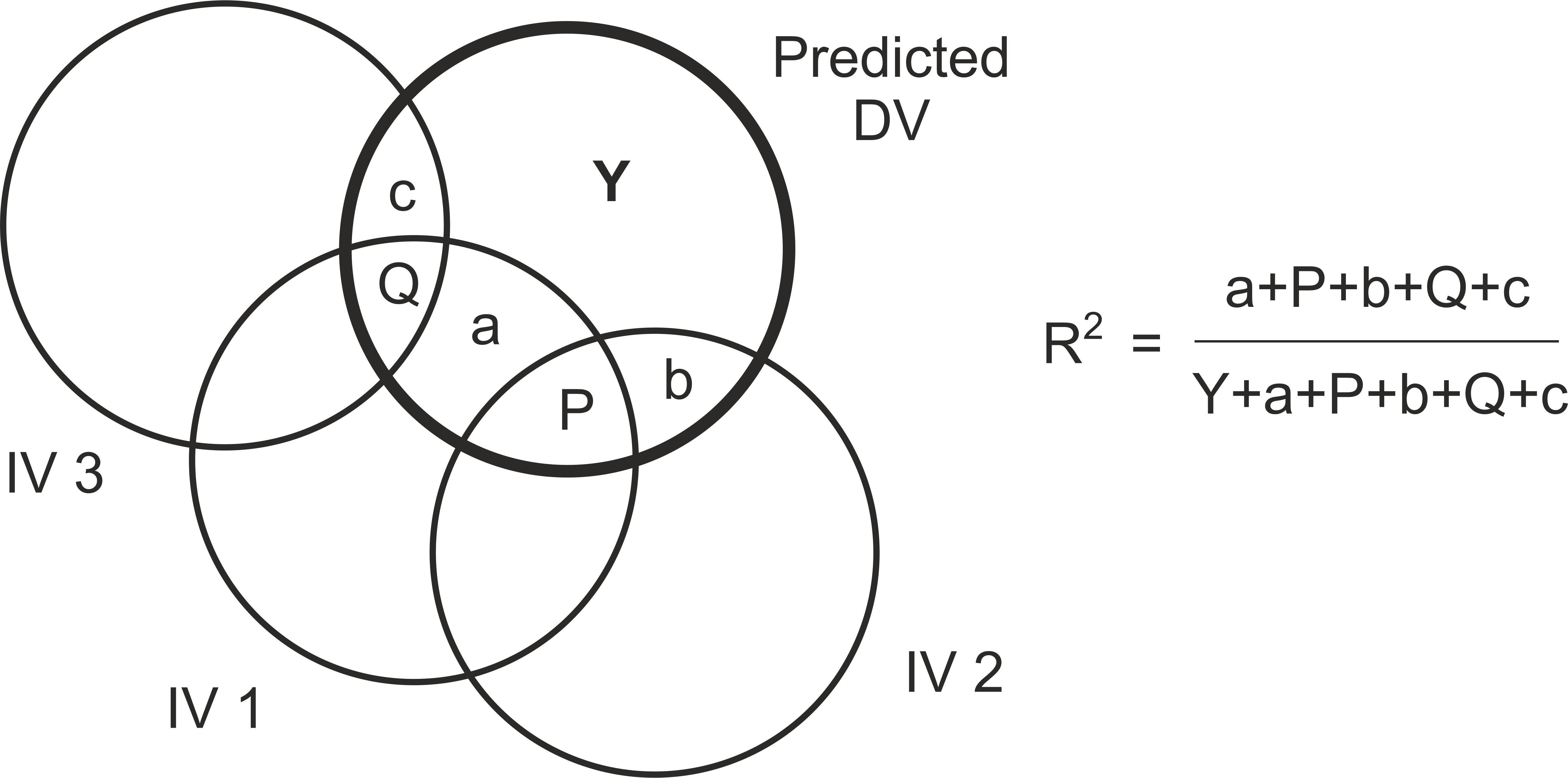
The zero order correlation is the "ordinary" correlation between two variables;  in the case of IV 1 and the DV, for example, it is r = .55.  Their partial correlation is .41, and their semi-partial or part correlation is .36.  Beta is .42, and is usually similar in value to the partial correlation.

As IVs are added to the regression equation we generally see the gradual reduction in the Beta weight for an IV.  Figure 4 illustrates how each additional IV some some variance in common with the other IVs and hence their unique contribution to the DV decreases.  Notice how region "a" has shrunk with the addition of IV 3.

Figure 4.  Venn diagram with 3 IVs

(§2) It could be said that continued reference to "Predicted DV" is unnecessary since almost everything said about this hypothetical variable applies just as well to the DV itself.  Nevertheless, we continue with this terminology because it aids the application of a number of regression principles in our introduction to factor analysis, where a factor is very much a hypothetical variable.  Of course, just mutter "DV!" whenever you read "Predicted DV" if that makes you feel better.

Back to MLR, three IVs

The value of requesting a Forward or Stepwise regression method is that an IV is included in the prediction equation only if it accounts for a significant increase in the variance accounted for in the DV.  In addition, the sequence of inclusion into the equation gives the order of importance of the IVs.  Table 5 provides the details for Model 3, being the MLR with three predictors.

Table 4.  MLR statistics, three IVs

Dependent Variable: Interest in generating income through online activities

The three IVs, taken together, account for 37% of the variance in the DV (R²) an increase of 2% from Model 1.  The prediction equation in standardised units is now Eqn 3:

Eqn 3.    Predicted interest in online income = 0.43 × Update device + .22 × Evaluate info + .14 × Right to use income

Our hypothetical variable "Predicted DV" correlates R = .61 with the DV.  The newly-included third IV, Right to use income, has a Beta of .14 with Predicted DV.  There are two matters to consider.  One is that Right to use income was only 7th or so in the order of IVs with the highest correlations with the DV, so what is it doing as the 3rd most important variable in the MLR?  Two is that .14 is a rather modest Beta, so do we have a genuinely important contribution to the variance accounted for?

An IV has a low r with the DV, how can it become a significant predictor?

We remember our introduction earlier:  MLR identifies the next IV as the one sharing the most "left over" variance with the DV.  That is, having accounted for the share of the variance shown by the IVs so far, MLR seeks an IV which accounts for variance not yet accounted for.  (Here is a clue if you have been looking at the zero-order, partial, and part correlations in the table of MLR statistics -- the next most useful IV is the one with the highest part correlation.  Review the definition of "sr" in Figure 3 to understand why.)  The IVs of Evaluate info and Update device also correlate significantly with Report or Block, Submit forms, Post videos, Peer support, and Freedom of phone use, and so the variance shared by these latter IVs with the DV is already accounted for by Evaluate info and Update device.  The left over variance not accounted for so far is shared with Right to use income (IV 3), a variable which does not correlate very highly with the latter IVs.  This makes IV 3 a significant contributor.

Does a significant beta make for an important contribution?

From our work with statistics so far, we already know that a statistically significant result is not necessarily a practically important result.  A large enough sample size ensures significance in the smallest of differences or for the smallest of associations.  This seems particularly true when working with associations -- r, R, or Chi-squared (§3).

To give the necessary practical perspective, it is now a usual editorial requirement for most journals to require reporting the effect size for every significant effect.  In the context of MLR, R, r, and Beta are themselves measures of effect size when squared, representing the proportion of variance accounted for, and are interpreted by convention (§4) as 1%, 10%, or 25% for small, medium, and large.  Where r or Beta = .14, r² or Beta² is around 2% -- small.

(§3) No, I don't know why this is.  My experience is that experimental studies have always given me more confidence in the practical importance of their significant results than observational studies.

(§4) See https://en.wikipedia.org/wiki/Effect_size

MLR, four IVs

The forward regression terminates with Model 4, being the MLR with four predictors, Table 5.  None of the remaining IVs reach the required p value of .05 or less for inclusion.

Table 5.  MLR statistics, four predictors

Dependent Variable: Interest in generating income through online activities

The four IVs, taken together, account for 39% of the variance in the DV (R²), an increase of 2% from Model 3.  The prediction equation in standardised units is now Eqn 4:

Eqn 4.    Predicted interest in online income = 0.39 × Update device + .17 × Evaluate info + .14 × Right to use income + .14 × Submit forms

Our hypothetical variable "Predicted DV" correlates R = .62 with the DV.

Summary

Our interest is in establishing which IVs are significantly associated with the DV.  From Table 5, we can say that, while most of the IVs have significant correlations with the DV, only four significantly account for variation in the DV not otherwise accounted for -- Update device (15%), Evaluate info (3%), Right to use income (2%), and Submit forms (2%) -- where (x%) is Beta² representing the proportion of variance uniquely accounted for.

We have constructed a hypothetical variable, Predicted interest in online income, composed so that it correlates with the DV, Interest in generating income through online activities, by weighting the contributions of the IVs in such a way that no other weighting or combination of IVs gives a higher correlation.

©2025 Lester Gilbert