These are the pages relevant to the topic of factor analysis:  Regression.  Introduction to principal components analysis.  Orthogonal factor rotation.  Oblique rotation.  This page, PCA full extraction.  Principle Axes extraction.  Cluster analysis.

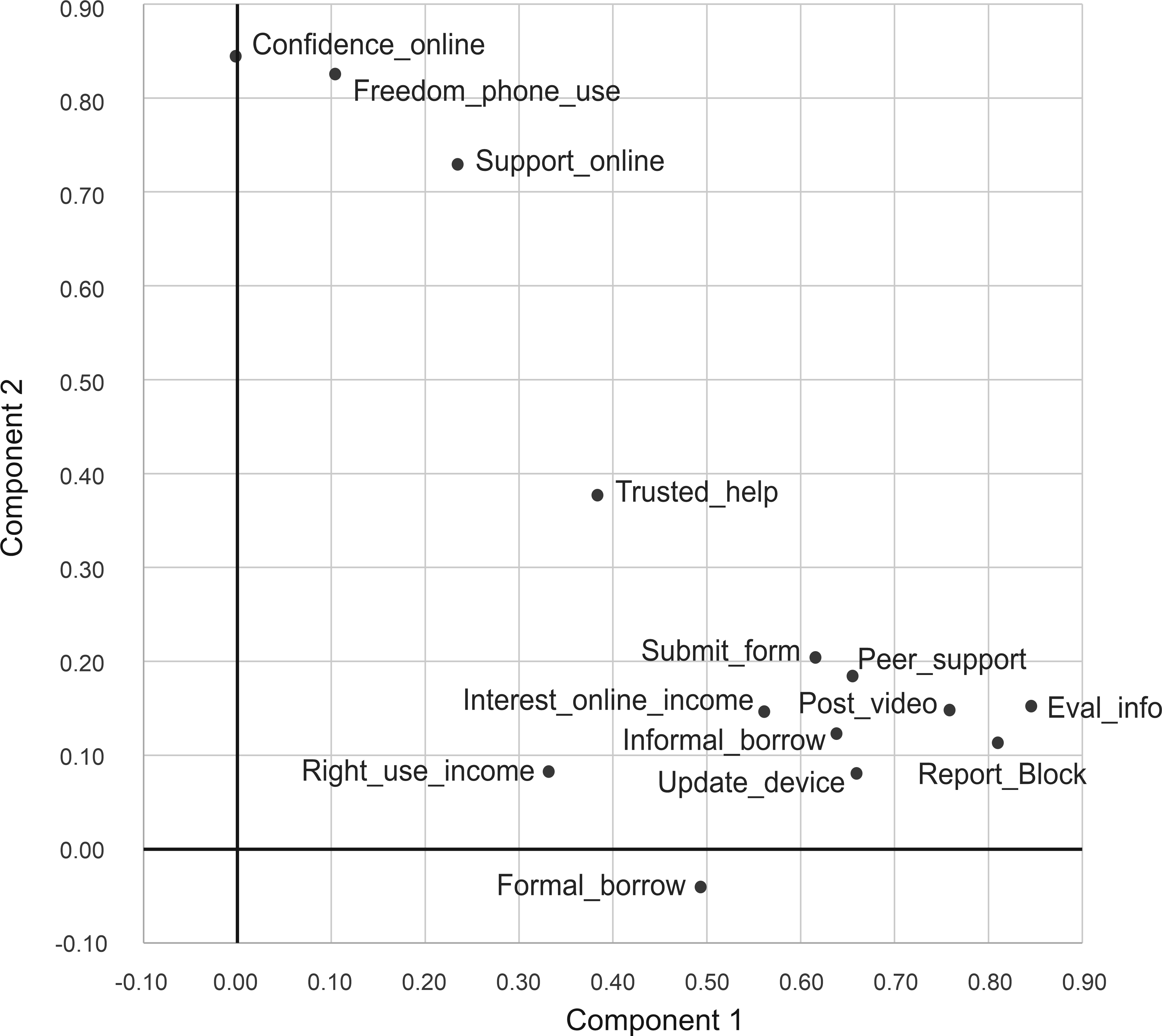
More than two factors

We ended the previous page (FA PCA orthog.htm) with two components extracted and orthogonally rotated and the feeling that, "While the two clusters of variables seem to have been more clearly identified, there remains the relative difficulty of interpreting Component 1 which incorporates a variety of themes."  Figure 1 shows the components in orthogonally-rotated space, and Table 1 shows the components matrix.

Figure 1.  Component plot in orthogonally-rotated space

Table 2.  Two components extracted, rotated, sorted, and edited

We extracted and orthogonally rotated 2 components following inspection of the scree plot, which seemed to show the scree starting at the third component.  On the other hand, we noticed that there were four components with Eigenvalues greater than 1, which is the other common rule of thumb for deciding the number of components to extract.  Here we'll extract and rotate four components.

Four components extracted

Table 3.  Communalities following 4 component extraction

We may notice that variables with very modest communalities after the extraction of two components now have substantial communalities.  For example, Right to use income has h² increased from .12 to .54.

Table 4.  Total variance explained

We notice that the four components account for 65.1% of the variance in the correlation matrix.

Table 5.  Extracted components matrix

There is no very good reason to show Table 5 because we will immediately rotate it (Varimax with Kaiser normalization);  there is usually little -- a polite way of saying, "absolutely nothing" -- to be gained by attempting to interpret extracted but un-rotated components.  We can pause, however, and for example notice that Right to use income, previously without substantial loadings, now loads substantially (our rule of thumb here is a loading greater than 0.4) on the fourth component.

Table 6.  Four components (orthogonally) rotated, sorted, and edited

We have arrived at the kind of table you will hopefully see for all your factor analyses -- clear variable clusters with substantial loadings on separate components and a minimum number of variables showing loadings on more than one component.

Interpreting the rotated components

Orthogonality.  It is important to remember that the four components each account for variance in the variables that is not accounted for by other components -- the rotation was orthogonal.  We see Component 1 comprises the various abilities to work online, along with Interest in online income, and it could be called "Online capabilities".  This Component is independent of, and is not connected to, Component 2 which might be called "General confidence, freedom, and support" or Component 4 which might be called "Specific freedoms and support for income generation".

Cross loadings (a).  Some connection between components can be seen in Table 6, where Component 3 might be called "Finances" and is dominated by borrowing, but it also has some loadings from two variables of Component 1 which might represent "Security".  Our rule of thumb is to omit loadings below 0.4.  This not carved in stone, it is a guideline.  You could decide (always explaining this with a note) to omit loadings below 0.5.  In this case, the "Security" loadings disappear from Component 3....  But see the oblique rotation, below.

Cross loadings (b).  The extraction of four components was by a rule of thumb.  There may be a good reason to extract and rotate five components to see if the "Security" variables could load on a separate component.

Causation and "marker" variables.  We warn against any lines of argument which seek to deduce causation from observational studies.  On the other hand....  Of all these variables, one stands out as "not like the others" -- Interest in online income.  It is a variable to which the other variables might contribute, and it would be an interesting research question for this data set to identify which of the variables would seem to support -- be related to -- interest in online income.  Part of the answer is nicely given by the factor analysis, which is "Online capabilities" of Component 1 because of the loading of this variable on that Component, and part of the answer is also given by the factor analysis -- not so much Components 2 or 4 which concern specific or general freedoms and support, but maybe some contribution from Component 3 finances.  Variables "not like the others" can be used as "marker" variables to aid the interpretation of a factor structure.  Common marker variables include demographic indicators such as education level, age, and so on.

No plots.  The rotated components occupy a four-dimensional space which makes them more or less impossible to visualize.  It is possible to construct plots of pairs of components -- there would be 6 plots -- but in practice the editing and sorting of loadings shown in Table 6 permits an adequate conceptualisation.

Obliquely rotated components

For interest, we rotate our four components obliquely (Oblimin with Kaiser normalization) instead of orthogonally.  Table 7 and 8 give the resulting pattern matrix and component correlations.

Table 7.  Four components (oblique rotation) pattern matrix, sorted, and edited

Table 8.  Component correlation matrix

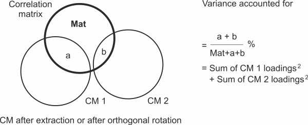
Interpreting the oblique components

The oblique rotation has obligingly taken the modest loadings of the two "Security" variables off Component 3, so that is a welcome outcome.  The rest of the pattern matrix loadings are similar to the orthogonal matrix of loadings.  Some variables show slightly higher loadings, some slightly lower, but all load in the same way on the same components.

Previously, we noted that the four orthogonally rotated components each accounted for variance in the variables that was not accounted for by other components.  We reproduce the Venn diagram from the page dealing with orthogonal rotation, Figure 2 here.  We see that Component 1, for example, accounts for region "a" of the variance in the correlation matrix of all the variables, and that Component 2 accounts for a separate region "b" that has no overlap with Component 1.

Figure 2.  Venn diagram of variance accounted for by orthogonal components

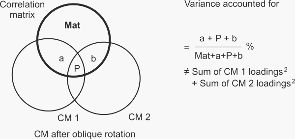
What of the obliquely rotated components?  We reproduce the Venn diagram from the page dealing with oblique rotation, Figure 3 here.  We see that Component 1, for example, accounts for region "a" of the variance in the correlation matrix of all the variables, and that Component 2 accounts for a separate region "b" that has no overlap with Component 1.  BUT we also see that there is a region "P" which both components share in accounting for the variance in the correlation matrix of all the variables.

Figure 3.  Venn diagram of the variance accounted for by oblique components

So an oblique component accounts for variance in the variables that is not accounted for by the other oblique components, just like orthogonal components.  BUT these are different regions of variance!  An oblique component accounts for unique variance, a/(Mat+a)%, in the way that a Beta weight accounts for unique variance in a regression equation, while an orthogonal component accounts for variance, (a+P)/(Mat+a+P+b)% in the way that a correlation coefficient accounts for common variance.  In order to restore the complete picture of variance accounted for in an oblique rotation, we must also reference the correlation between the oblique components (Table 8).

In the oblique rotation, we see Component 1, comprising the various abilities to work online, along with an Interest in online income, called "Online capabilities", as before, is correlated with Component 2 "General confidence, freedom, and support", r = .24;  is correlated with Component 3 "Finances", r = .31;  and is correlated with Component 4 "Specific freedoms and support for income generation", r = .26.  Ah.  Furthermore, Component 2 "General confidence, freedom, and support" is correlated with Component 3 "Finances", r = .15;  Component 2 is correlated with Component 4 "Specific freedoms and support for income generation", r = .17;  and Component 3 "Finances" is correlated with Component 4 "Specific freedoms and support for income generation", r = .23.  Hmmm.  Phew!

These oblique component correlations are modest.  The largest is r = .31 between Component 1 and Component 3, representing a shared variance of 10%.  By comparison, the largest loading in Component 1 is .84, representing 71%, so there is some basis for suggesting that the modest component correlations can be ignored while benefiting from the clearer picture given by the pattern matrix to support interpreting what seem to be the 4 components which mainly account for the correlations seen in the 14-variable correlation matrix.  While you may need some good luck with that in your viva or thesis defence, it is a line of argument that a reviewer should find acceptable in a journal article.

©2025 Lester Gilbert